POLYNOMIAL REGRESSION
LINEAR VS NON-LINEAR REGRESSION
INTRODUCTION :
In this blog we will see how to fit a perfect plane for a dataset . Sometimes it’s sufficient to fit Linear plane . But for sometimes it’s not sufficient to get the good accuracy score by fitting a linear plane . At that condition we go for a Non-Linear plane that best fits our dataset .
We will see which best fits either linear or non-linear plane for our simple dataset for better understanding .


So the above dataframe is our dataset . In which there are 6 rows and 2 columns named 0 and 1 . In which 0 is independent variable and 1 is the dependent variable .If we draw a scatter plot between dependent variable and independent variable . From our naked eye itself we can surely say we can’t fit a straight line for our dataset .
But for better understanding we will fit the best Linear line that better fit’s our dataset to predict the dependent variable.
FITTING A LINEAR PLANE :


Hence , the above fit is the best linear fit for our dataset . In which we can clearly see the linear line is not actually able to fit this dataset .
So,
Y = 2.06 * (independent variable) -2.6599999
Above function is not a best equation for our model that fits our data .We can also see that the predicted values by our model for 1 is -0.6 and for 11 it predicted 9.7 . The variance is more in our case .
We need to reduce the variance for that we will go for non-linear fit .
INTUITION POLYNOMIAL REGRESSION:
So , before going into the code for fitting a polynomial regression model . I just wanted to give a intuition about how polynomial regression works
At first we fitted a linear line for that the we used a equation of a line as ,
Y = M*X + C (for one independent variable in our case)
OR
Y = M1*X1 + M2*X2 + ….. +MnXn + C (for n independent variable straight plane )
where M1,M2….Mn are slopes and X1,X2,……Xn are attributes
But to fit a Non-linear say curve . We just need to raise the power of independent variable
like ,
Degree 2: Y = M1*X² + M2*X + C (Where the X is the independent variable)
Degree 3: Y = M1*X³ + M3*X² + C
This we will now dive into code

From above we can clearly see that xpoly has been changed and as been raised to the powers . Like ,
IV = independent variable
Y = M*(1’s matrix) + M1*(IV) + M2*(IV)² + M3*(IV)³ + C
As from xpoly , It is now not like before dateframe it will have excess of attributes than the it .
That we can clearly see ,
- First column has 1’s
- Second column has the given independent variable
- Third column has the squared values of Independent variable
- Fourth column has cubed of Independent variable
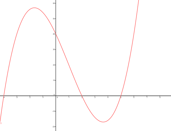
The above equation will fit a curve like this ,

We will see what curve to fit in our dataset ,


Hence , this curve best fit’s our dataset perfectly . There is a little bit of variance yet that won’t bather at all .
Best fit curve is ,
Y = 0 * (column 0) — 1.2775 *(column 1) + 0.4767 *(column 2) + 1.7899999
We can also see that the predicted values by our model for 1 is 0.986 and for 11 it predicted 11.28 . The variance is less in this case .
Finding the Optimal Intercept and Co-efficient is clearly explained in this blog :
https://medium.com/@kkarthikeyanvk/guide-to-simply-explained-linear-974da3d3c4f
This is how the POLYNOMIAL REGRESSION works !
CHEERS !!!
