Understanding The Formula: Normal Distribution

The normal distribution is crucial in statistics and machine learning because many real-world datasets naturally follow this distribution, allowing us to make accurate predictions and inferences. In statistics, it is the foundation for key techniques like hypothesis testing, confidence intervals, and regression analysis, which rely on the assumption of normally distributed errors. In machine learning, algorithms like linear regression, logistic regression, and Gaussian Naive Bayes perform optimally when features are normally distributed. Several machine learning algorithms rely on the assumption that the data is normally distributed for optimal performance. For instance, Linear Regression and Logistic Regression assume that the residuals (errors) follow a normal distribution, which is essential for accurate hypothesis testing and confidence intervals. Gaussian Naive Bayes explicitly assumes that features are normally distributed to calculate probabilities. Similarly, Linear Discriminant Analysis (LDA) assumes that data from each class follows a Gaussian distribution with different means but equal variance. Principal Component Analysis (PCA) also performs better when data is normally distributed, as it captures maximum variance. Additionally, Support Vector Machines (SVM) with RBF kernel and K-Nearest Neighbors (KNN) work more effectively when data distribution is Gaussian due to the nature of distance-based calculations. When the data is not normally distributed, transformations like log transformation or Box-Cox transformation can help improve model performance.

Moreover, the Central Limit Theorem (CLT) states that the distribution of sample means approaches a normal distribution as the sample size increases, regardless of the original data distribution. This property allows us to use a normal distribution for making probabilistic assumptions and building robust models, even when working with small datasets.

Laymen Term Explanation

The normal distribution, also known as the Gaussian distribution, is a fundamental concept in statistics and machine learning. It is a bell-shaped, symmetric probability distribution where most data points cluster around the mean, with fewer values appearing as you move further from the center. The distribution is fully defined by two parameters: the mean (μ), which represents the center, and the standard deviation (σ), which measures the spread. The 68–95–99.7 rule states that approximately 68% of data falls within one standard deviation from the mean, 95% within two, and 99.7% within three. As it can be seen in the below image.

Fig 1: Bell Curve (Source)

Formula

The formula for normal distribution:

Fig 2: Formula (Source)

What does each variable in the formula?

f(x) represents the probability density
σ represents the variance of the data
π represents the mathematical pie value
μ represents the mean of the data

Understanding the formula step by step

Part I: Let us focus on the below formula for now and understand what it exactly means.
This is the core part of the normal distribution formula, which is:

What does this part do?

This part is responsible for shaping the bell curve.

It controls how the probability decreases as you move away from the mean (μ). See fig 1.

Let’s Understand Step-by-step:

The exponential function e−x shrinks very quickly as x increases.

• If x=μ, this part becomes 1 (because e⁰=1).
• If x is far from μ, this part shrinks very fast towards 0.
• (x−μ): This measures how far the point x is from the mean μ.
• Squaring it, (x−μ)2, makes sure the distance is always positive (because distance can’t be negative).
• Dividing by 2σ^2: This controls how spread out the curve is, depending on the variance.

Now lets deep dive into the formula further:

So, If not considering the exponential for now. The remaining part is the square of the Z-score.

Why Square of Z-Score?

• Squaring makes both the left and right sides of the curve equal (symmetry).
• Without squaring, it wouldn’t be a bell curve.

The plot of the square of the z-score is:

Fig 3: Square of the Z-score

From the above graph, the x-axis is the data points and y is the Z-score. As you see the Z-score is not bound to a limit it varies from negative infinity to positive. When we plot the frequency of Z-scores for all data points, it naturally forms a bell curve.

Why are we dividing by 2?

(x−μ)^2 \2σ^2

In probability theory, squaring alone grows too fast.

• Dividing by 2 slows down the growth.
• This comes from Gaussian mathematics and calculus-based derivation.
• In higher-level math, this division by 2 comes from the variance of the distribution.

Why are we doing the exponential of Z-score squared divided by 2?

This is THE MOST IMPORTANT PART of the normal distribution!

The exponential function is used to “punish” extreme points.

What does “punishing” mean here?

• In a normal distribution, most data points are close to the mean (μ).
• Data points that are too far from the mean should have a very low probability.
• The exponential function ensures that these extreme values get very small weights (probabilities). See fig 1.

Fig 4: Exponential of the squared Z-score

What do you observe?

• The highest value is exactly at the mean (x=μ), where the probability is 1.
• As you move away from the mean, the probability rapidly drops to almost zero.
• The drop is smooth and symmetric on both sides, thanks to the squared Z-score.

What is happening here?

The exponential function is “punishing” extreme values, so:

• Points near the mean get a high probability.
• Points far from the mean get crushed to nearly zero.

How will be the Plot when the standard deviation varies?

Fig 5: Exponential part of normal distribution for different sigmas.

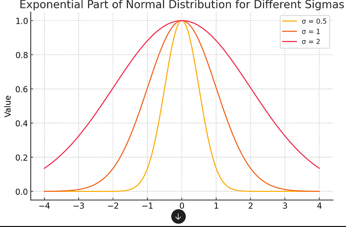
• When σ is small, the exponential function punishes extreme values more harshly, making the curve very steep.
• When σ is large, the punishment is slow, allowing more data points to spread out.
• This is exactly how the normal distribution controls the spread of data.
• By changing σ, you control the “tightness” of the bell curve

Part II: Now will understand the below part in the formula.

Which can also be interpreted as below:

What does it do?

In probability distributions, the total area under the curve must be exactly 1, because the total probability of all possible outcomes is 1.

• This part ensures that the total area under the bell curve is exactly 1, which is a key property of any probability distribution.
• It scales the curve so that the probabilities calculated from the distribution are valid and add up to 1.
• Without this factor, the curve might be too high or too low, leading to incorrect probabilities.

Mathematical Proof (Using Integration):

The integral of the normal distribution is:

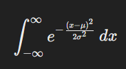
The result of this integral is:

So, to balance this out and make the area = 1, we divide by the same value.
This part normalizes the curve, ensuring that the total probability is exactly 1, which is a core requirement of any probability distribution.

Hope this article explains the intuition of normal distribution formula. Cheers!